Refer to Exhibit 10-5. When Te Is $300 Billion, What Will Firms Most Likely Firms Do Next?

28.2 The Aggregate Expenditures Model

Learning Objectives

1. Explain and illustrate the amass expenditures model and the concept of equilibrium real Gdp.
2. Distinguish between democratic and induced aggregate expenditures and explicate why a modify in democratic expenditures leads to a multiplied change in equilibrium real Gdp.
3. Discuss how adding taxes, government purchases, and net exports to a simplified amass expenditures model affects the multiplier and hence the touch on on real Gdp that arises from an initial change in autonomous expenditures.

The consumption role relates the level of consumption in a period to the level of dispensable personal income in that flow. In this section, nosotros incorporate other components of amass demand: investment, government purchases, and net exports. In doing and so, we shall develop a new model of the conclusion of equilibrium real GDP, the aggregate expenditures model. This model relates aggregate expenditures, which equal the sum of planned levels of consumption, investment, regime purchases, and net exports at a given price level, to the level of real GDP. Nosotros shall see that people, firms, and regime agencies may not always spend what they had planned to spend. If so, then actual existent GDP will not be the same as aggregate expenditures, and the economy will not be at the equilibrium level of real GDP.

One purpose of examining the aggregate expenditures model is to gain a deeper understanding of the "ripple furnishings" from a change in one or more than components of aggregate demand. As we saw in the chapter that introduced the aggregate demand and aggregate supply model, a alter in investment, government purchases, or internet exports leads to greater product; this creates additional income for households, which induces additional consumption, leading to more production, more income, more consumption, and and then on. The aggregate expenditures model provides a context inside which this series of ripple effects tin can be better understood. A second reason for introducing the model is that we tin apply it to derive the aggregate need curve for the model of aggregate need and amass supply.

To run across how the aggregate expenditures model works, we begin with a very simplified model in which there is neither a government sector nor a strange sector. Then we use the findings based on this simplified model to build a more realistic model. The equations for the simplified economy are easier to work with, and we can readily apply the conclusions reached from analyzing a simplified economic system to draw conclusions most a more realistic 1.

The Aggregate Expenditures Model: A Simplified View

To develop a simple model, we assume that there are only 2 components of amass expenditures: consumption and investment. In the affiliate on measuring total output and income, we learned that existent gross domestic product and existent gross domestic income are the same thing. With no regime or foreign sector, gross domestic income in this economy and disposable personal income would exist nearly the aforementioned. To simplify further, we volition assume that depreciation and undistributed corporate profits (retained earnings) are cipher. Thus, for this case, we presume that disposable personal income and real GDP are identical.

Finally, we shall also assume that the simply component of aggregate expenditures that may non be at the planned level is investment. Firms determine a level of investment they intend to brand in each menstruation. The level of investment firms intend to brand in a flow is called planned investment. Some investment is unplanned. Suppose, for example, that firms produce and await to sell more than appurtenances during a period than they actually sell. The unsold goods will be added to the firms' inventories, and they volition thus be counted as part of investment. Unplanned investment is investment during a period that firms did not intend to brand. It is also possible that firms may sell more than they had expected. In this case, inventories will fall below what firms expected, in which case, unplanned investment would exist negative. Investment during a menstruation equals the sum of planned investment (I _P) and unplanned investment (I _U).

Equation 28.6

[latex]I = I_P + I_U[/latex]

Nosotros shall observe that planned and unplanned investment play key roles in the aggregate expenditures model.

Democratic and Induced Aggregate Expenditures

Economists distinguish 2 types of expenditures. Expenditures that do not vary with the level of real Gdp are called autonomous amass expenditures. In our example, we presume that planned investment expenditures are autonomous. Expenditures that vary with existent Gross domestic product are chosen induced aggregate expenditures. Consumption spending that rises with real GDP is an example of an induced aggregate expenditure. Figure 28.6 "Autonomous and Induced Aggregate Expenditures" illustrates the difference between democratic and induced aggregate expenditures. With real GDP on the horizontal axis and aggregate expenditures on the vertical axis, democratic aggregate expenditures are shown as a horizontal line in Console (a). A curve showing induced aggregate expenditures has a slope greater than zero; the value of an induced amass expenditure changes with changes in real Gdp. Panel (b) shows induced aggregate expenditures that are positively related to real GDP.

Figure 28.6 Autonomous and Induced Aggregate Expenditures

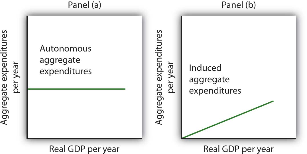
Autonomous aggregate expenditures practice not vary with the level of real Gdp; induced amass expenditures exercise. Autonomous amass expenditures are shown by the horizontal line in Panel (a). Induced aggregate expenditures vary with real Gross domestic product, as in Panel (b).

Democratic and Induced Consumption

The concept of the marginal propensity to consume suggests that consumption contains induced aggregate expenditures; an increase in existent GDP raises consumption. Merely consumption contains an autonomous component too. The level of consumption at the intersection of the consumption function and the vertical axis is regarded as autonomous consumption; this level of spending would occur regardless of the level of real GDP.

Consider the consumption office we used in deriving the schedule and curve illustrated in Figure 28.two "Plotting a Consumption Function":

[latex]C = \$ 300 \: billion + 0.8Y[/latex]

Nosotros tin can omit the subscript on disposable personal income because of the simplifications nosotros have made in this section, and the symbol Y tin can be thought of as representing both disposable personal income and GDP. Considering we presume that the toll level in the amass expenditures model is constant, Gdp equals existent GDP. At every level of real Gdp, consumption includes $300 billion in democratic aggregate expenditures. It will also contain expenditures "induced" by the level of real Gross domestic product. At a level of real GDP of $2,000 billion, for example, consumption equals $1,900 billion: $300 billion in autonomous aggregate expenditures and $1,600 billion in consumption induced by the $two,000 billion level of existent Gross domestic product.

Figure 28.7 "Autonomous and Induced Consumption" illustrates these two components of consumption. Autonomous consumption, C _a, which is ever $300 billion, is shown in Panel (a); its equation is

Equation 28.vii

[latex]C_a = \$ 300 \: billion[/latex]

Induced consumption C _i is shown in Panel (b); its equation is

Equation 28.viii

[latex]C_i = 0.8Y[/latex]

The consumption office is given by the sum of Equation 28.7 and Equation 28.8; it is shown in Console (c) of Figure 28.7 "Democratic and Induced Consumption". Information technology is the same every bit the equation C = $300 billion + 0.8Y _d, since in this unproblematic example, Y and Y _d are the same.

Figure 28.vii Democratic and Induced Consumption

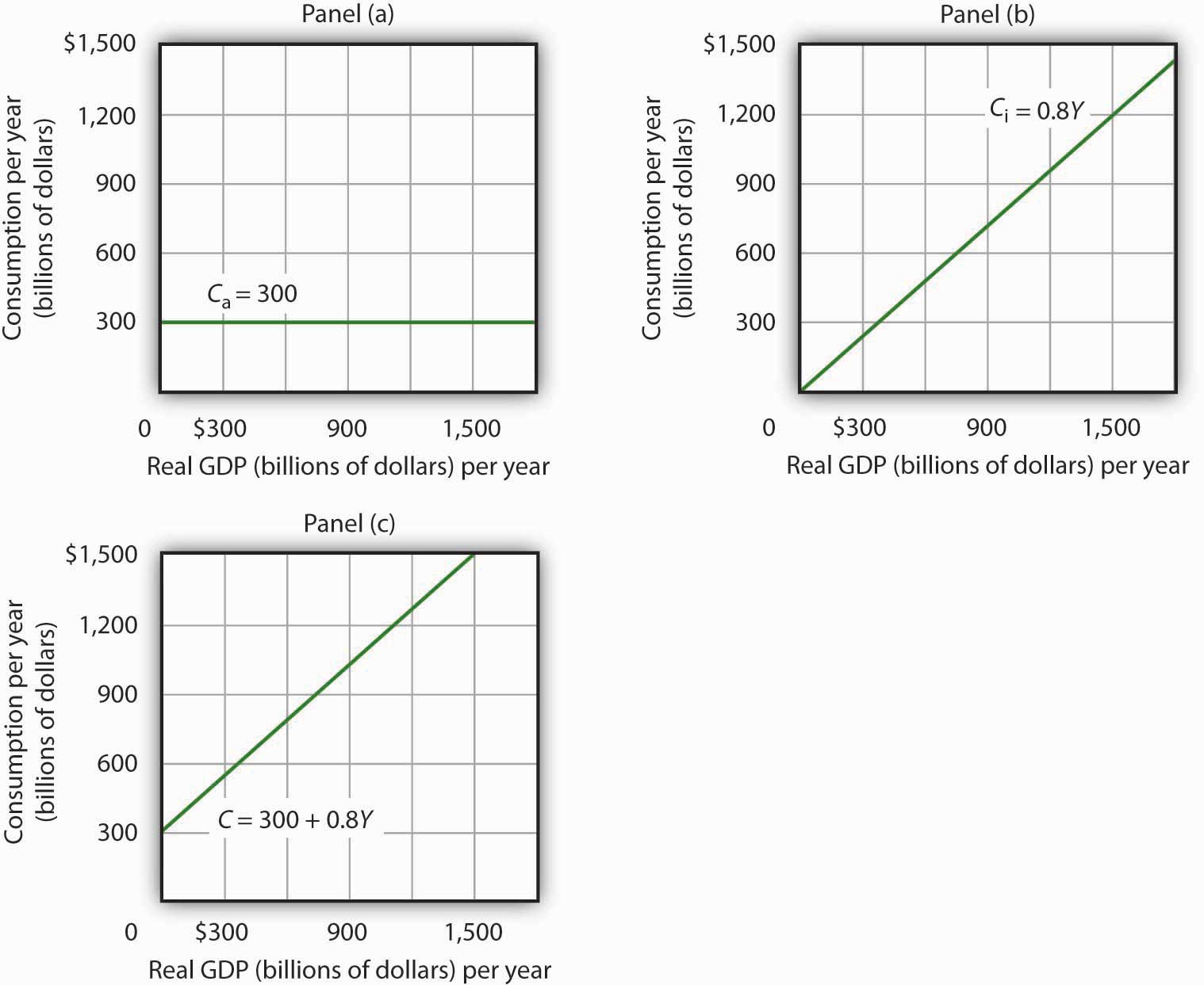
Consumption has an autonomous component and an induced component. In Console (a), autonomous consumption C _a equals $300 billion at every level of real Gross domestic product. Panel (b) shows induced consumption C _i. Full consumption C is shown in Console (c).

Plotting the Aggregate Expenditures Curve

In this simplified economy, investment is the only other component of aggregate expenditures. We shall assume that investment is autonomous and that firms programme to invest $1,100 billion per year.

Equation 28.9

[latex]I_P = \$ 1,100 \: billion[/latex]

The level of planned investment is unaffected by the level of existent GDP.

Aggregate expenditures equal the sum of consumption C and planned investment I _P. The aggregate expenditures function is the relationship of aggregate expenditures to the value of real GDP. Information technology can exist represented with an equation, as a table, or as a bend.

We begin with the definition of amass expenditures AE when there is no government or foreign sector:

Equation 28.10

[latex]AE = C + I_P[/latex]

Substituting the information from above on consumption and planned investment yields (throughout this discussion all values are in billions of base-year dollars)

[latex]AE = \$ 300 + 0.8Y + \$ one,100[/latex]

or

Equation 28.11

[latex]AE = \$ one,400 + 0.8Y[/latex]

Equation 28.xi is the algebraic representation of the aggregate expenditures role. We shall use this equation to determine the equilibrium level of existent Gdp in the aggregate expenditures model. It is important to keep in mind that aggregate expenditures mensurate full planned spending at each level of real Gross domestic product (for any given cost level). Real Gdp is total production. Aggregate expenditures and existent Gross domestic product need not exist equal, and indeed will not be equal except when the economy is operating at its equilibrium level, as nosotros will see in the adjacent section.

In Equation 28.11, the autonomous component of aggregate expenditures is $1,400 billion, and the induced component is 0.8Y. We shall plot this aggregate expenditures function. To do so, we arbitrarily select various levels of real Gross domestic product and so use Equation 28.x to compute aggregate expenditures at each level. At a level of real Gross domestic product of $half-dozen,000 billion, for example, aggregate expenditures equal $6,200 billion:

[latex]AE = \$ 1,400 + 0.8 \: ( \$ 6,000) = \$ 6,200[/latex]

The table in Effigy 28.viii "Plotting the Amass Expenditures Curve" shows the values of aggregate expenditures at various levels of real Gdp. Based on these values, we plot the aggregate expenditures bend. To obtain each value for aggregate expenditures, we but insert the corresponding value for real Gross domestic product into Equation 28.11. The value at which the aggregate expenditures curve intersects the vertical axis corresponds to the level of autonomous amass expenditures. In our example, autonomous aggregate expenditures equal $one,400 billion. That figure includes $ane,100 billion in planned investment, which is assumed to be autonomous, and $300 billion in autonomous consumption expenditure.

Effigy 28.8 Plotting the Amass Expenditures Curve

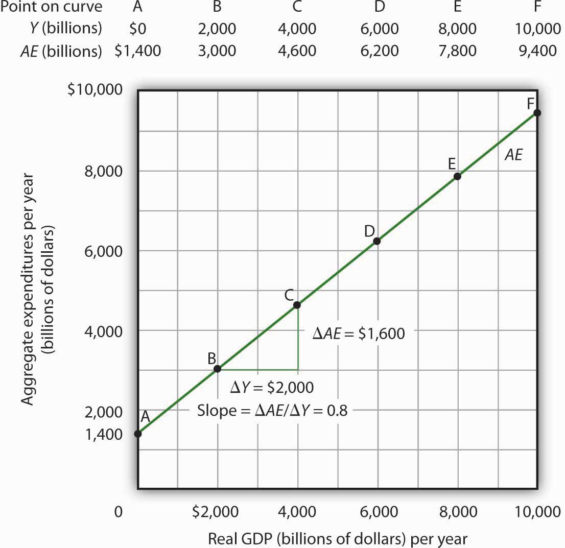
Values for aggregate expenditures AE are computed by inserting values for real GDP into Equation 28.10; these are given in the amass expenditures schedule. The betoken at which the aggregate expenditures bend intersects the vertical centrality is the value of autonomous aggregate expenditures, hither $1,400 billion. The slope of this aggregate expenditures curve is 0.eight.

The Gradient of the Aggregate Expenditures Curve

The slope of the aggregate expenditures curve, given by the alter in aggregate expenditures divided past the change in real Gross domestic product between whatever two points, measures the additional expenditures induced past increases in real GDP. The slope for the aggregate expenditures bend in Figure 28.eight "Plotting the Aggregate Expenditures Curve" is shown for points B and C: it is 0.8.

In Figure 28.8 "Plotting the Amass Expenditures Bend", the slope of the aggregate expenditures curve equals the marginal propensity to consume. This is considering nosotros have assumed that the merely other expenditure, planned investment, is autonomous and that real GDP and disposable personal income are identical. Changes in real GDP thus touch on only consumption in this simplified economy.

Equilibrium in the Amass Expenditures Model

Real Gross domestic product is a mensurate of the total output of firms. Aggregate expenditures equal total planned spending on that output. Equilibrium in the model occurs where amass expenditures in some period equal real Gross domestic product in that flow. One way to remember about equilibrium is to recognize that firms, except for some inventory that they plan to hold, produce appurtenances and services with the intention of selling them. Amass expenditures consist of what people, firms, and regime agencies programme to spend. If the economy is at its equilibrium real GDP, so firms are selling what they plan to sell (that is, there are no unplanned changes in inventories).

Figure 28.nine "Determining Equilibrium in the Aggregate Expenditures Model" illustrates the concept of equilibrium in the aggregate expenditures model. A 45-degree line connects all the points at which the values on the two axes, representing amass expenditures and real Gross domestic product, are equal. Equilibrium must occur at some indicate along this 45-degree line. The point at which the amass expenditures curve crosses the 45-degree line is the equilibrium real Gross domestic product, here accomplished at a existent Gdp of $seven,000 billion.

Effigy 28.9 Determining Equilibrium in the Amass Expenditures Model

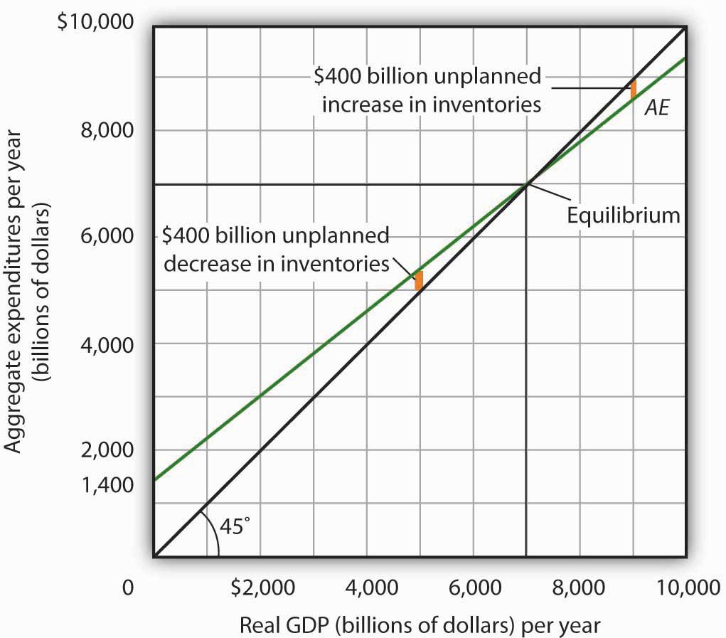
The 45-caste line shows all the points at which aggregate expenditures AE equal existent GDP, as required for equilibrium. The equilibrium solution occurs where the AE bend crosses the 45-degree line, at a real GDP of $7,000 billion.

Equation 28.11 tells us that at a existent Gross domestic product of $vii,000 billion, the sum of consumption and planned investment is $7,000 billion—precisely the level of output firms produced. At that level of output, firms sell what they planned to sell and keep inventories that they planned to keep. A existent Gdp of $7,000 billion represents equilibrium in the sense that information technology generates an equal level of aggregate expenditures.

If firms were to produce a real Gross domestic product greater than $seven,000 billion per twelvemonth, aggregate expenditures would autumn short of existent Gdp. At a level of real Gross domestic product of $9,000 billion per yr, for example, aggregate expenditures equal $8,600 billion. Firms would be left with $400 billion worth of goods they intended to sell but did non. Their bodily level of investment would be $400 billion greater than their planned level of investment. With those unsold goods on hand (that is, with an unplanned increase in inventories), firms would be likely to cut their output, moving the economy toward its equilibrium GDP of $7,000 billion. If firms were to produce $five,000 billion, aggregate expenditures would exist $5,400 billion. Consumers and firms would demand more than was produced; firms would respond by reducing their inventories below the planned level (that is, there would be an unplanned decrease in inventories) and increasing their output in subsequent periods, again moving the economy toward its equilibrium existent Gdp of $7,000 billion. Figure 28.10 "Adjusting to Equilibrium Real Gdp" shows possible levels of real Gdp in the economy for the amass expenditures role illustrated in Effigy 28.nine "Determining Equilibrium in the Aggregate Expenditures Model". It shows the level of aggregate expenditures at various levels of real Gross domestic product and the direction in which real GDP will alter whenever AE does not equal real Gdp. At any level of real Gross domestic product other than the equilibrium level, at that place is unplanned investment.

Figure 28.10 Adjusting to Equilibrium Real Gross domestic product

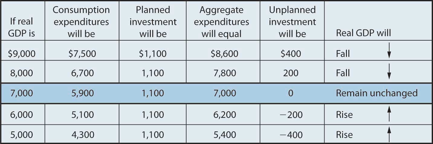
Each level of existent GDP will result in a detail amount of amass expenditures. If amass expenditures are less than the level of real Gdp, firms volition reduce their output and existent GDP volition autumn. If aggregate expenditures exceed real Gdp, then firms will increment their output and real GDP will rise. If aggregate expenditures equal real GDP, then firms will leave their output unchanged; we take achieved equilibrium in the amass expenditures model. At equilibrium, there is no unplanned investment. Here, that occurs at a real Gdp of $7,000 billion.

Changes in Amass Expenditures: The Multiplier

In the amass expenditures model, equilibrium is found at the level of existent Gross domestic product at which the aggregate expenditures curve crosses the 45-caste line. It follows that a shift in the curve volition change equilibrium real Gross domestic product. Hither we will examine the magnitude of such changes.

Effigy 28.xi "A Modify in Autonomous Aggregate Expenditures Changes Equilibrium Real Gdp" begins with the aggregate expenditures curve shown in Effigy 28.9 "Determining Equilibrium in the Aggregate Expenditures Model". At present suppose that planned investment increases from the original value of $ane,100 billion to a new value of $1,400 billion—an increase of $300 billion. This increment in planned investment shifts the aggregate expenditures bend up by $300 billion, all other things unchanged. Find, however, that the new amass expenditures bend intersects the 45-caste line at a real GDP of $eight,500 billion. The $300 billion increase in planned investment has produced an increase in equilibrium real Gdp of $one,500 billion.

Figure 28.xi A Alter in Democratic Aggregate Expenditures Changes Equilibrium Real GDP

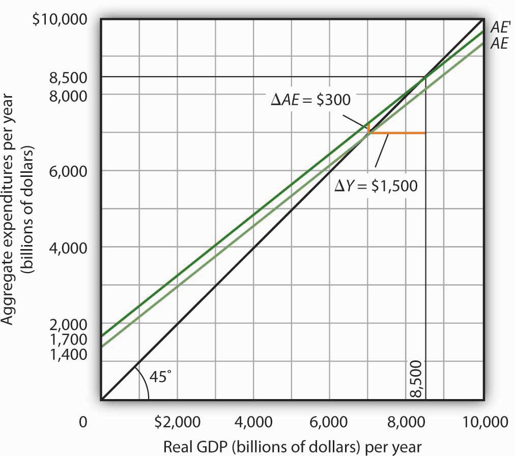
An increase of $300 billion in planned investment raises the amass expenditures curve by $300 billion. The $300 billion increase in planned investment results in an increase in equilibrium real GDP of $1,500 billion.

How could an increment in aggregate expenditures of $300 billion produce an increase in equilibrium real Gross domestic product of $1,500 billion? The answer lies in the operation of the multiplier. Considering firms have increased their demand for investment goods (that is, for capital) past $300 billion, the firms that produce those goods volition have $300 billion in additional orders. They volition produce $300 billion in additional real Gdp and, given our simplifying assumption, $300 billion in additional disposable personal income. But in this economy, each $1 of additional existent GDP induces $0.80 in boosted consumption. The $300 billion increase in autonomous aggregate expenditures initially induces $240 billion (= 0.8 × $300 billion) in additional consumption.

The $240 billion in boosted consumption boosts production, creating some other $240 billion in existent Gdp. But that second round of increment in existent Gross domestic product induces $192 billion (= 0.8 × $240) in boosted consumption, creating still more production, still more income, and still more than consumption. Somewhen (subsequently many additional rounds of increases in induced consumption), the $300 billion increase in amass expenditures will result in a $i,500 billion increase in equilibrium real Gdp. Table 28.1 "The Multiplied Effect of an Increase in Democratic Aggregate Expenditures" shows the multiplied effect of a $300 billion increase in autonomous aggregate expenditures, assuming each $1 of additional existent GDP induces $0.80 in boosted consumption.

Tabular array 28.ane The Multiplied Upshot of an Increase in Autonomous Aggregate Expenditures

Round of spending	Increase in real Gdp (billions of dollars)
1	$300
2	240
3	192
4	154
5	123
half-dozen	98
vii	79
8	63
9	fifty
10	forty
11	32
12	26
Subsequent rounds	+103
Total increase in real GDP	$1,500

The size of the additional rounds of expenditure is based on the slope of the aggregate expenditures function, which in this example is simply the marginal propensity to consume. Had the gradient been flatter (if the marginal propensity to consume were smaller), the additional rounds of spending would have been smaller. A steeper slope would mean that the additional rounds of spending would accept been larger.

This process could also work in contrary. That is, a decrease in planned investment would lead to a multiplied decrease in existent Gdp. A reduction in planned investment would reduce the incomes of some households. They would reduce their consumption by the MPC times the reduction in their income. That, in turn, would reduce incomes for households that would have received the spending past the first grouping of households. The procedure continues, thus multiplying the impact of the reduction in aggregate expenditures resulting from the reduction in planned investment.

Computation of the Multiplier

The multiplier is the number by which we multiply an initial modify in aggregate demand to go the full amount of the shift in the aggregate demand curve. Considering the multiplier shows the amount by which the amass demand curve shifts at a given price level, and the aggregate expenditures model assumes a given price level, nosotros can use the aggregate expenditures model to derive the multiplier explicitly.

Let Y _eq exist the equilibrium level of existent Gdp in the aggregate expenditures model, and allow A be autonomous aggregate expenditures. Then the multiplier is

Equation 28.12

[latex]Multiplier = \frac{ \Delta Y_{eq}}{ \Delta \bar{A}}[/latex]

In the example nosotros have just discussed, a alter in autonomous amass expenditures of $300 billion produced a change in equilibrium existent Gdp of $1,500 billion. The value of the multiplier is therefore $1,500/$300 = 5.

The multiplier event works because a change in autonomous aggregate expenditures causes a change in real GDP and dispensable personal income, inducing a further change in the level of amass expenditures, which creates still more GDP and thus an even higher level of amass expenditures. The caste to which a given change in existent GDP induces a change in aggregate expenditures is given in this simplified economic system by the marginal propensity to swallow, which, in this example, is the slope of the amass expenditures curve. The slope of the aggregate expenditures curve is thus linked to the size of the multiplier. Nosotros turn now to an investigation of the human relationship between the marginal propensity to consume and the multiplier.

The Marginal Propensity to Eat and the Multiplier

We can compute the multiplier for this simplified economy from the marginal propensity to consume. We know that the corporeality by which equilibrium existent Gross domestic product volition change as a upshot of a change in aggregate expenditures consists of two parts: the change in autonomous aggregate expenditures itself, Δ $$ \bar{A} $$, and the induced change in spending. This induced alter equals the marginal propensity to consume times the change in equilibrium existent GDP, ΔY _eq. Thus

Equation 28.13

[latex]\Delta Y_{eq} = \Delta \bar{A} + MPC \Delta Y_{eq}[/latex]

Decrease the MPCΔY _eq term from both sides of the equation:

[latex]\Delta Y_{eq} \: - \: MPC \Delta Y_{eq} = \Delta \bar{A}[/latex]

Gene out the ΔY _eq term on the left:

[latex]\Delta Y_{eq} (one \: - \: MPC) = \Delta \bar{A}[/latex]

Finally, solve for the multiplier ΔYeq/Δ$$ \bar{A} $$ past dividing both sides of the equation higher up by ΔA and by dividing both sides by (1 − MPC). We get the post-obit:

Equation 28.14

[latex]\frac{ \Delta Y_{eq}}{ \Delta \bar{A}} = \frac{1}{1 \: - \: MPC}[/latex]

We thus compute the multiplier by taking 1 minus the marginal propensity to consume, then dividing the issue into 1. In our example, the marginal propensity to consume is 0.8; the multiplier is 5, as nosotros have already seen [multiplier = 1/(1 − MPC) = one/(ane − 0.viii) = 1/0.2 = v]. Since the sum of the marginal propensity to consume and the marginal propensity to salve is ane, the denominator on the correct-hand side of Equation 28.thirteen is equivalent to the MPS, and the multiplier could also exist expressed as 1/MPS.

Equation 28.15

[latex]Multiplier = \frac{1}{MPS}[/latex]

We tin rearrange terms in Equation 28.14 to use the multiplier to compute the impact of a change in democratic aggregate expenditures. We simply multiply both sides of the equation by $$ \bar{A} $$ to obtain the following:

Equation 28.sixteen

[latex]\Delta Y_{eq} = \frac{ \Delta \bar{A}}{i \: - \: MPC}[/latex]

The change in the equilibrium level of income in the amass expenditures model (call up that the model assumes a constant toll level) equals the change in autonomous amass expenditures times the multiplier. Thus, the greater the multiplier, the greater will exist the impact on income of a change in autonomous amass expenditures.

The Aggregate Expenditures Model in a More Realistic Economy

Four conclusions emerge from our application of the amass expenditures model to the simplified economy presented and then far. These conclusions tin be practical to a more than realistic view of the economic system.

1. The aggregate expenditures function relates aggregate expenditures to existent Gdp. The intercept of the amass expenditures bend shows the level of autonomous amass expenditures. The slope of the amass expenditures curve shows how much increases in real GDP induce additional aggregate expenditures.
2. Equilibrium real GDP occurs where aggregate expenditures equal existent GDP.
3. A change in autonomous aggregate expenditures changes equilibrium existent GDP past a multiple of the change in autonomous amass expenditures.
4. The size of the multiplier depends on the gradient of the amass expenditures curve. The steeper the amass expenditures curve, the larger the multiplier; the flatter the aggregate expenditures curve, the smaller the multiplier.

These four points still concord equally we add together the ii other components of aggregate expenditures—government purchases and net exports—and recognize that authorities non only spends merely too collects taxes. We look beginning at the effect of adding taxes to the aggregate expenditures model and then at the effect of adding government purchases and net exports.

Taxes and the Amass Expenditure Role

Suppose that the only divergence between existent Gdp and dispensable personal income is personal income taxes. Let us run across what happens to the slope of the amass expenditures function.

Every bit before, nosotros assume that the marginal propensity to consume is 0.viii, but nosotros at present add the assumption that income taxes have ¼ of real Gross domestic product. This means that for every additional $one of real Gdp, disposable personal income rises by $0.75 and, in turn, consumption rises by $0.60 (= 0.8 × $0.75). In the simplified model in which disposable personal income and real GDP were the same, an boosted $1 of real GDP raised consumption by $0.80. The gradient of the aggregate expenditures bend was 0.8, the marginal propensity to eat. Now, as a consequence of taxes, the aggregate expenditures curve volition be flatter than the one shown in Figure 28.8 "Plotting the Amass Expenditures Curve" and Effigy 28.10 "Adjusting to Equilibrium Real Gross domestic product". In this example, the slope volition be 0.half-dozen; an boosted $1 of real GDP will increase consumption past $0.60.

Other things the same, the multiplier volition be smaller than information technology was in the simplified economic system in which disposable personal income and real Gdp were identical. The wedge betwixt dispensable personal income and real Gdp created past taxes means that the additional rounds of spending induced past a alter in autonomous aggregate expenditures will exist smaller than if there were no taxes. Hence, the multiplied issue of any alter in democratic aggregate expenditures is smaller.

The Addition of Government Purchases and Net Exports

Suppose that government purchases and net exports are autonomous. If and so, they enter the aggregate expenditures function in the same mode that investment did. Compared to the simplified aggregate expenditures model, the amass expenditures bend shifts up by the amount of regime purchases and net exports¹.

Figure 28.12 "The Aggregate Expenditures Role: Comparison of a Simplified Economy and a More than Realistic Economy" shows the difference betwixt the amass expenditures model of the simplified economic system in Figure 28.9 "Determining Equilibrium in the Amass Expenditures Model" and a more than realistic view of the economic system. Panel (a) shows an AE curve for an economy with only consumption and investment expenditures. In Console (b), the AE curve includes all four components of aggregate expenditures.

Figure 28.12 The Aggregate Expenditures Function: Comparison of a Simplified Economy and a More than Realistic Economy

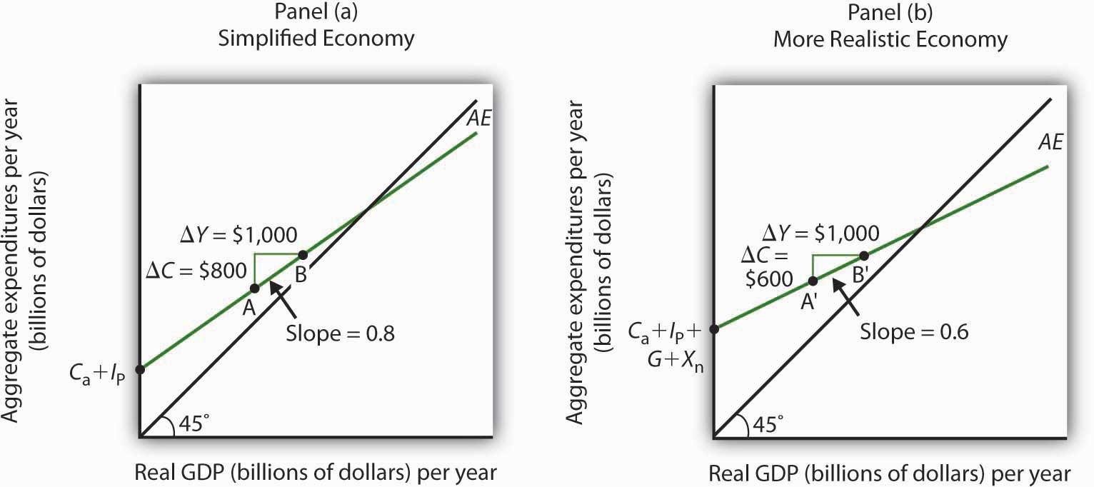
Panel (a) shows an aggregate expenditures curve for a simplified view of the economic system; Console (b) shows an aggregate expenditures curve for a more realistic model. The AE bend in Panel (b) has a higher intercept than the AE curve in Panel (a) because of the boosted components of autonomous aggregate expenditures in a more than realistic view of the economy. The slope of the AE curve in Panel (b) is flatter than the slope of the AE curve in Panel (a). In a simplified economic system, the slope of the AE bend is the marginal propensity to consume (MPC). In a more realistic view of the economy, it is less than the MPC considering of the difference between real GDP and disposable personal income.

There are two major differences between the aggregate expenditures curves shown in the two panels. Notice commencement that the intercept of the AE curve in Panel (b) is higher than that of the AE curve in Panel (a). The reason is that, in addition to the autonomous office of consumption and planned investment, there are two other components of amass expenditures—regime purchases and net exports—that nosotros have also assumed are autonomous. Thus, the intercept of the aggregate expenditures curve in Panel (b) is the sum of the four autonomous aggregate expenditures components: consumption (C _a), planned investment (I _P), regime purchases (1000), and net exports (X _northward). In Panel (a), the intercept includes only the offset ii components.

Second, notice that the slope of the aggregate expenditures curve is flatter for the more realistic economy in Panel (b) than it is for the simplified economy in Panel (a). This tin be seen past comparing the slope of the amass expenditures curve between points A and B in Panel (a) to the slope of the aggregate expenditures curve betwixt points A′ and B′ in Panel (b). Betwixt both sets of points, real Gross domestic product changes by the aforementioned amount, $1,000 billion. In Panel (a), consumption rises past $800 billion, whereas in Console (b) consumption rises past only $600 billion. This divergence occurs because, in the more than realistic view of the economic system, households take only a fraction of real Gdp available as dispensable personal income. Thus, for a given change in real GDP, consumption rises by a smaller amount.

Allow us examine what happens to equilibrium existent Gdp in each case if there is a shift in democratic aggregate expenditures, such as an increase in planned investment, as shown in Figure 28.13 "A Alter in Autonomous Amass Expenditures: Comparison of a Simplified Economy and a More Realistic Economy". In both panels, the initial level of equilibrium real GDP is the same, Y ₁. Equilibrium real GDP occurs where the given aggregate expenditures curve intersects the 45-caste line. The aggregate expenditures curve shifts up by the same amount—ΔA is the same in both panels. The new level of equilibrium real Gross domestic product occurs where the new AE curve intersects the 45-degree line. In Panel (a), we see that the new level of equilibrium real Gdp rises to Y ₂, but in Console (b) information technology rises only to Y ₃. Since the same change in autonomous amass expenditures led to a greater increase in equilibrium real GDP in Panel (a) than in Panel (b), the multiplier for the more than realistic model of the economy must be smaller. The multiplier is smaller, of course, because the slope of the aggregate expenditures curve is flatter.

Figure 28.13 A Modify in Autonomous Amass Expenditures: Comparison of a Simplified Economy and a More Realistic Economy

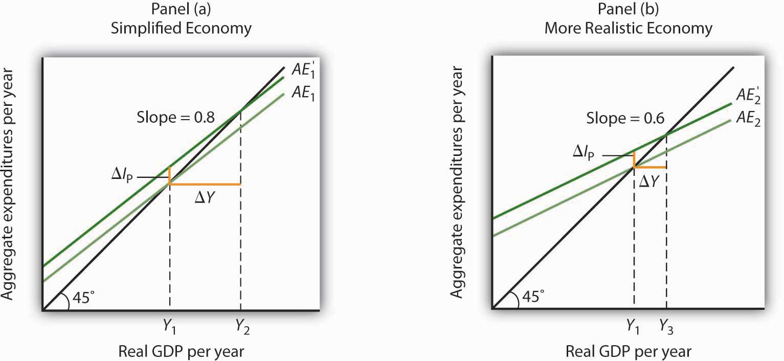
In Panels (a) and (b), equilibrium real Gross domestic product is initially Y ₁. Then autonomous aggregate expenditures rise by the aforementioned amount, ΔI _P. In Panel (a), the upward shift in the AE bend leads to a new level of equilibrium real GDP of Y _two; in Console (b) equilibrium real GDP rises to Y ₃. Because equilibrium real GDP rises by more in Console (a) than in Console (b), the multiplier in the simplified economy is greater than in the more than realistic i.

Cardinal Takeaways

• The aggregate expenditures model relates aggregate expenditures to real GDP. Equilibrium in the model occurs where amass expenditures equal real Gdp and is found graphically at the intersection of the amass expenditures bend and the 45-degree line.
• Economists distinguish between democratic and induced aggregate expenditures. The former practise not vary with Gdp; the latter practice.
• Equilibrium in the amass expenditures model implies that unintended investment equals zero.
• A change in autonomous amass expenditures leads to a modify in equilibrium existent GDP, which is a multiple of the change in autonomous aggregate expenditures.
• The size of the multiplier depends on the slope of the aggregate expenditures curve. In general, the steeper the aggregate expenditures curve, the greater the multiplier. The flatter the aggregate expenditures bend, the smaller the multiplier.
• Income taxes tend to flatten the aggregate expenditures curve.

Try Information technology!

Suppose you lot are given the post-obit data for an economy. All data are in billions of dollars. Y is actual real Gdp, and C, I _P, G, and X _n are the consumption, planned investment, regime purchases, and cyberspace exports components of aggregate expenditures, respectively.

Y	C	I p	One thousand	X n
$0	$800	$1,000	$1,400	−$200
two,500	2,300	1,000	1,400	−200
5,000	3,800	i,000	1,400	−200
7,500	5,300	one,000	1,400	−200
10,000	half dozen,800	1,000	one,400	−200

1. Plot the corresponding amass expenditures bend and draw in the 45-degree line.
2. What is the intercept of the AE curve? What is its slope?
3. Decide the equilibrium level of real Gross domestic product.
4. Now suppose that internet exports autumn by $ane,000 billion and that this is the only alter in autonomous amass expenditures. Plot the new amass expenditures curve. What is the new equilibrium level of real Gross domestic product?
5. What is the value of the multiplier?

Case in Point: Fiscal Policy in the Kennedy Administration

Information technology was the first fourth dimension expansionary fiscal policy had ever been proposed. The economy had slipped into a recession in 1960. Presidential candidate John Kennedy received proposals from several economists that year for a tax cutting aimed at stimulating the economy. Every bit a candidate, he was unconvinced. Merely, as president he proposed the tax cut in 1962. His chief economic adviser, Walter Heller, defended the tax cut idea before Congress and introduced what was politically a novel concept: the multiplier.

In testimony to the Senate Subcommittee on Employment and Manpower, Mr. Heller predicted that a $10 billion cut in personal income taxes would boost consumption "past over $nine billion."

To assess the ultimate bear on of the taxation cutting, Mr. Heller practical the aggregate expenditures model. He rounded the increased consumption off to $9 billion and explained,

"This is far from the end of the matter. The higher production of consumer goods to meet this extra spending would mean actress employment, higher payrolls, higher profits, and higher farm and professional and service incomes. This added purchasing power would generate even so further increases in spending and incomes. … The initial ascension of $nine billion, plus this extra consumption spending and extra output of consumer goods, would add over $eighteen billion to our annual Gdp."

We tin can summarize this continuing process by saying that a "multiplier" of approximately two has been applied to the direct increment of consumption spending.

Mr. Heller too predicted that proposed cuts in corporate income taxation rates would increase investment by most $six billion. The full change in democratic amass expenditures would thus be $fifteen billion: $9 billion in consumption and $half dozen billion in investment. He predicted that the total increase in equilibrium GDP would be $30 billion, the amount the Quango of Economic Advisers had estimated would exist necessary to reach full employment.

In the end, the tax cut was non passed until 1964, later President Kennedy'south assassination in 1963. While the Quango of Economic Directorate concluded that the tax cutting had worked as advertised, it came long after the economic system had recovered and tended to push the economy into an inflationary gap. Every bit we volition run across in afterwards chapters, the tax cutting helped push button the economy into a period of rising inflation.

Source: Economic Report of the President 1964 (Washington, DC: U.Southward. Regime Press Function, 1964), 172–73.

Answers to Try Information technology! Problems

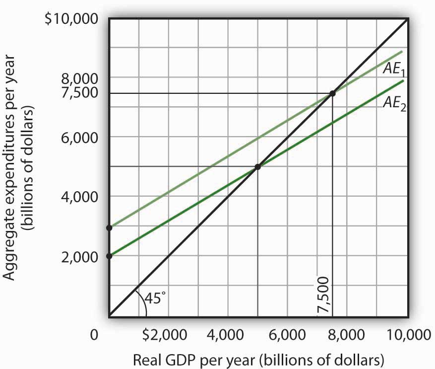
1. The aggregate expenditures bend is plotted in the accompanying chart as AE ₁.

2. The intercept of the AE _ane curve is $three,000. It is the amount of aggregate expenditures (C + I _P + G + X _{due north}) when real Gdp is zero. The slope of the AE ₁ curve is 0.6. It can exist constitute past determining the amount of aggregate expenditures for whatsoever two levels of real GDP and and then past dividing the change in aggregate expenditures by the change in real Gdp over the interval. For case, between existent Gross domestic product of $2,500 and $5,000, aggregate expenditures go from $4,500 to $vi,000. Thus,

   [latex]\frac{ \Delta E_1}{ \Delta Y} = \frac{ \$ 6,000 \: - \: \$ 4,500}{ \$ v,000 \: - \: \$ two,500} = \frac{ \$ 1,500}{ \$ two,500} = 0.6[/latex]

3. The equilibrium level of real Gdp is $7,500. Information technology can be found past determining the intersection of AE ₁ and the 45-caste line. At Y = $7,500, AE ₁ = $5,300 + one,000 + 1,400 − 200 = $7,500.
4. A reduction of internet exports of $1,000 shifts the aggregate expenditures curve down by $1,000 to AE _ii. The equilibrium real Gross domestic product falls from $7,500 to $5,000. The new aggregate expenditures bend, AE ₂, intersects the 45-degree line at real Gdp of $v,000.
5. The multiplier is 2.5 [= (−$2,500)/(−$ane,000)].

Figure 28.xv

¹An even more realistic view of the economic system might presume that imports are induced, since as a state'south real GDP rises it volition purchase more goods and services, some of which will exist imports. In that example, the slope of the amass expenditures curve would alter.

moosesearpon.blogspot.com

Source: https://open.lib.umn.edu/principleseconomics/chapter/28-2-the-aggregate-expenditures-model/

Share this post